Can You Find The Fish In State Names?
By Benjamin Soltoff in r
May 22, 2020
The recent Riddler classic offered this intriguing challenge:
Ohio is the only state whose name doesnt share any letters with the word “mackerel.” Its strange, but its true.
But that isnt the only pairing of a state and a word you can say that about — its not even the only fish! Kentucky has “goldfish” to itself, Montana has “jellyfish” and Delaware has “monkfish,” just to name a few.
What is the longest “mackerel?” That is, what is the longest word that doesnt share any letters with exactly one state? (If multiple “mackerels” are tied for being the longest, can you find them all?)
Extra credit: Which state has the most “mackerels?” That is, which state has the most words for which it is the only state without any letters in common with those words?
Given the provided dictionary, we need to find all the words that do not have overlapping letters with state names (specifically, mackerels are ones with exactly one state with which it does not share letters).
In order to do that, I tokenized each word at the character-level, then compared the list of dictionary words to all the state names to find all non-overlapping pairs of words.
library(tidyverse)
## ── Attaching packages ─────────────────────────────────────── tidyverse 1.3.1 ──
## ✓ ggplot2 3.3.3     ✓ purrr   0.3.4
## ✓ tibble  3.1.1     ✓ dplyr   1.0.6
## ✓ tidyr   1.1.3     ✓ stringr 1.4.0
## ✓ readr   1.4.0     ✓ forcats 0.5.1
## ── Conflicts ────────────────────────────────────────── tidyverse_conflicts() ──
## x dplyr::filter() masks stats::filter()
## x dplyr::lag()    masks stats::lag()
library(tidytext)

theme_set(theme_minimal(base_size = 18))
First we retrieve the dictionary of words. R already includes state names as the state.name constant.
# get list of words
all_words <- tibble(word = readLines("https://norvig.com/ngrams/word.list"))
states <- tibble(word = state.name)
Next I use tidytext::unnest_tokens() to tokenize at the character level. Since it doesn’t matter how many times the word uses a specific character, I just need each distinct appearance.1 From here I nest() the data frame so each word is a row and all their unique characters are in separate characte vectors.
# combine together
tokens <- bind_rows(
  all_words = all_words,
  states = states,
  .id = "source"
) %>%
  # tokenize by character
  unnest_tokens(
    output = letter,
    input = word,
    token = "characters",
    drop = FALSE
  ) %>%
  # remove duplicates
  distinct() %>%
  # store data as one row per word and all unique letters as character vectors
  nest(cols = c(letter)) %>%
  mutate(letters = map(cols, ~ .$letter)) %>%
  select(-cols) %>%
  # split by source
  group_split(source, keep = FALSE)
## Warning: The `keep` argument of `group_split()` is deprecated as of dplyr 1.0.0.
## Please use the `.keep` argument instead.
tokens
## <list_of<
##   tbl_df<
##     word   : character
##     letters: list
##   >
## >[2]>
## [[1]]
## # A tibble: 263,533 x 2
##    word     letters
##    <chr>    <list>
##  1 aa       <chr [1]>
##  2 aah      <chr [2]>
##  3 aahed    <chr [4]>
##  4 aahing   <chr [5]>
##  5 aahs     <chr [3]>
##  6 aal      <chr [2]>
##  7 aalii    <chr [3]>
##  8 aaliis   <chr [4]>
##  9 aals     <chr [3]>
## 10 aardvark <chr [5]>
## # … with 263,523 more rows
##
## [[2]]
## # A tibble: 50 x 2
##    word        letters
##    <chr>       <list>
##  1 Alabama     <chr [4]>
##  2 Alaska      <chr [4]>
##  3 Arizona     <chr [6]>
##  4 Arkansas    <chr [5]>
##  5 California  <chr [8]>
##  6 Colorado    <chr [6]>
##  7 Connecticut <chr [7]>
##  8 Delaware    <chr [6]>
##  9 Florida     <chr [7]>
## 10 Georgia     <chr [6]>
## # … with 40 more rows
From here, I need to form all possible combinations between each dictionary word and state name. expand.grid() lets me form all possible combinations, while a couple of left_join() operations bring together all the character tokens.
# form all possible cominations of the dictionary and state names
tokens_combo <- expand.grid(
  word_all = tokens[[1]]$word,
  word_state = tokens[[2]]$word
) %>%
  left_join(tokens[[1]], by = c("word_all" = "word")) %>%
  rename(letters_all = letters) %>%
  left_join(tokens[[2]], by = c("word_state" = "word")) %>%
  rename(letters_state = letters) %>%
  as_tibble()
tokens_combo
## # A tibble: 13,176,650 x 4
##    word_all word_state letters_all letters_state
##    <chr>    <chr>      <list>      <list>
##  1 aa       Alabama    <chr [1]>   <chr [4]>
##  2 aah      Alabama    <chr [2]>   <chr [4]>
##  3 aahed    Alabama    <chr [4]>   <chr [4]>
##  4 aahing   Alabama    <chr [5]>   <chr [4]>
##  5 aahs     Alabama    <chr [3]>   <chr [4]>
##  6 aal      Alabama    <chr [2]>   <chr [4]>
##  7 aalii    Alabama    <chr [3]>   <chr [4]>
##  8 aaliis   Alabama    <chr [4]>   <chr [4]>
##  9 aals     Alabama    <chr [3]>   <chr [4]>
## 10 aardvark Alabama    <chr [5]>   <chr [4]>
## # … with 13,176,640 more rows
The tricky part was finding the correct syntax to check all the characters in the dictionary word individually – if any of the letters could be found in the state name, we did not have a valid match. Combining %in% with the any() function allows us to do just that.
# only keep rows where the dictionary word does not have any letters in common
# with the state name
words_not_in_common <- tokens_combo %>%
  mutate(any_letters_in_common = map2_lgl(letters_all,
                                          letters_state,
                                          ~ any(.x %in% .y == TRUE))) %>%
  filter(!any_letters_in_common)
Turns out that even with millions of pairs to iterate through, it only took about 40 seconds to complete the comparisons on my computer.
From here, we just need to find all the mackerels and check their word length.
# check to see if a word has multiple mackerels
mackerels <- words_not_in_common %>%
  count(word_all) %>%
  # only keep words with a single mackerel
  filter(n == 1) %>%
  # what are their length?
  left_join(words_not_in_common) %>%
  mutate(length = map_dbl(word_all, nchar)) %>%
  select(-starts_with("letters"), -any_letters_in_common) %>%
  arrange(-length)
## Joining, by = "word_all"
# what are the longest mackerels?
mackerels %>%
  filter(length == max(length)) %>%
  knitr::kable(col.names = c(
    "Word", "Number of mackerels",
    "State", "Word length"
  ))
| Word | Number of mackerels | State | Word length |
|---|---|---|---|
| counterproductivenesses | 1 | Alabama | 23 |
| hydrochlorofluorocarbon | 1 | Mississippi | 23 |
2 words tie for the longest mackerel at 23 characters each.
As for the extra credit, which states have the most mackerels? Given what we already calculated, let’s instead aggregate total number of mackerels for each state.
# join with states info
state_mackerels <- mackerels %>%
  count(word_state) %>%
  # add back in states which have no mackerels
  full_join(states, by = c("word_state" = "word")) %>%
  mutate(n = ifelse(is.na(n), 0, n)) %>%
  arrange(-n, word_state)

ggplot(
  data = state_mackerels,
  mapping = aes(
    x = factor(word_state, levels = word_state) %>% fct_rev(),
    y = n
  )
) +
  geom_col() +
  coord_flip() +
  labs(
    title = "Number of mackerels by state",
    x = NULL,
    y = "Number of mackerels"
  )
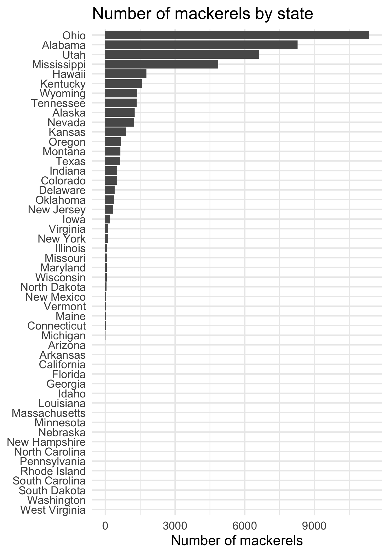
Ohio is the clear winner; rounding out the top four are Alabama, Utah, and Mississippi.
Session Info
devtools::session_info()
## ─ Session info ───────────────────────────────────────────────────────────────
##  setting  value
##  version  R version 4.0.4 (2021-02-15)
##  os       macOS Big Sur 10.16
##  system   x86_64, darwin17.0
##  ui       X11
##  language (EN)
##  collate  en_US.UTF-8
##  ctype    en_US.UTF-8
##  tz       America/Chicago
##  date     2021-06-01
##
## ─ Packages ───────────────────────────────────────────────────────────────────
##  package     * version date       lib source
##  assertthat    0.2.1   2019-03-21 [1] CRAN (R 4.0.0)
##  backports     1.2.1   2020-12-09 [1] CRAN (R 4.0.2)
##  blogdown      1.3     2021-04-14 [1] CRAN (R 4.0.2)
##  bookdown      0.22    2021-04-22 [1] CRAN (R 4.0.2)
##  broom         0.7.6   2021-04-05 [1] CRAN (R 4.0.4)
##  bslib         0.2.5   2021-05-12 [1] CRAN (R 4.0.4)
##  cachem        1.0.5   2021-05-15 [1] CRAN (R 4.0.2)
##  callr         3.7.0   2021-04-20 [1] CRAN (R 4.0.2)
##  cellranger    1.1.0   2016-07-27 [1] CRAN (R 4.0.0)
##  cli           2.5.0   2021-04-26 [1] CRAN (R 4.0.2)
##  colorspace    2.0-1   2021-05-04 [1] CRAN (R 4.0.2)
##  crayon        1.4.1   2021-02-08 [1] CRAN (R 4.0.2)
##  DBI           1.1.1   2021-01-15 [1] CRAN (R 4.0.2)
##  dbplyr        2.1.1   2021-04-06 [1] CRAN (R 4.0.4)
##  desc          1.3.0   2021-03-05 [1] CRAN (R 4.0.2)
##  devtools      2.4.1   2021-05-05 [1] CRAN (R 4.0.2)
##  digest        0.6.27  2020-10-24 [1] CRAN (R 4.0.2)
##  dplyr       * 1.0.6   2021-05-05 [1] CRAN (R 4.0.2)
##  ellipsis      0.3.2   2021-04-29 [1] CRAN (R 4.0.2)
##  evaluate      0.14    2019-05-28 [1] CRAN (R 4.0.0)
##  fansi         0.4.2   2021-01-15 [1] CRAN (R 4.0.2)
##  fastmap       1.1.0   2021-01-25 [1] CRAN (R 4.0.2)
##  forcats     * 0.5.1   2021-01-27 [1] CRAN (R 4.0.2)
##  fs            1.5.0   2020-07-31 [1] CRAN (R 4.0.2)
##  generics      0.1.0   2020-10-31 [1] CRAN (R 4.0.2)
##  ggplot2     * 3.3.3   2020-12-30 [1] CRAN (R 4.0.2)
##  glue          1.4.2   2020-08-27 [1] CRAN (R 4.0.2)
##  gtable        0.3.0   2019-03-25 [1] CRAN (R 4.0.0)
##  haven         2.4.1   2021-04-23 [1] CRAN (R 4.0.2)
##  here          1.0.1   2020-12-13 [1] CRAN (R 4.0.2)
##  hms           1.1.0   2021-05-17 [1] CRAN (R 4.0.4)
##  htmltools     0.5.1.1 2021-01-22 [1] CRAN (R 4.0.2)
##  httr          1.4.2   2020-07-20 [1] CRAN (R 4.0.2)
##  janeaustenr   0.1.5   2017-06-10 [1] CRAN (R 4.0.0)
##  jquerylib     0.1.4   2021-04-26 [1] CRAN (R 4.0.2)
##  jsonlite      1.7.2   2020-12-09 [1] CRAN (R 4.0.2)
##  knitr         1.33    2021-04-24 [1] CRAN (R 4.0.2)
##  lattice       0.20-44 2021-05-02 [1] CRAN (R 4.0.2)
##  lifecycle     1.0.0   2021-02-15 [1] CRAN (R 4.0.2)
##  lubridate     1.7.10  2021-02-26 [1] CRAN (R 4.0.2)
##  magrittr      2.0.1   2020-11-17 [1] CRAN (R 4.0.2)
##  Matrix        1.3-3   2021-05-04 [1] CRAN (R 4.0.2)
##  memoise       2.0.0   2021-01-26 [1] CRAN (R 4.0.2)
##  modelr        0.1.8   2020-05-19 [1] CRAN (R 4.0.0)
##  munsell       0.5.0   2018-06-12 [1] CRAN (R 4.0.0)
##  pillar        1.6.1   2021-05-16 [1] CRAN (R 4.0.4)
##  pkgbuild      1.2.0   2020-12-15 [1] CRAN (R 4.0.2)
##  pkgconfig     2.0.3   2019-09-22 [1] CRAN (R 4.0.0)
##  pkgload       1.2.1   2021-04-06 [1] CRAN (R 4.0.2)
##  prettyunits   1.1.1   2020-01-24 [1] CRAN (R 4.0.0)
##  processx      3.5.2   2021-04-30 [1] CRAN (R 4.0.2)
##  ps            1.6.0   2021-02-28 [1] CRAN (R 4.0.2)
##  purrr       * 0.3.4   2020-04-17 [1] CRAN (R 4.0.0)
##  R6            2.5.0   2020-10-28 [1] CRAN (R 4.0.2)
##  Rcpp          1.0.6   2021-01-15 [1] CRAN (R 4.0.2)
##  readr       * 1.4.0   2020-10-05 [1] CRAN (R 4.0.2)
##  readxl        1.3.1   2019-03-13 [1] CRAN (R 4.0.0)
##  remotes       2.3.0   2021-04-01 [1] CRAN (R 4.0.2)
##  reprex        2.0.0   2021-04-02 [1] CRAN (R 4.0.2)
##  rlang         0.4.11  2021-04-30 [1] CRAN (R 4.0.2)
##  rmarkdown     2.8     2021-05-07 [1] CRAN (R 4.0.2)
##  rprojroot     2.0.2   2020-11-15 [1] CRAN (R 4.0.2)
##  rstudioapi    0.13    2020-11-12 [1] CRAN (R 4.0.2)
##  rvest         1.0.0   2021-03-09 [1] CRAN (R 4.0.2)
##  sass          0.4.0   2021-05-12 [1] CRAN (R 4.0.2)
##  scales        1.1.1   2020-05-11 [1] CRAN (R 4.0.0)
##  sessioninfo   1.1.1   2018-11-05 [1] CRAN (R 4.0.0)
##  SnowballC     0.7.0   2020-04-01 [1] CRAN (R 4.0.0)
##  stringi       1.6.1   2021-05-10 [1] CRAN (R 4.0.2)
##  stringr     * 1.4.0   2019-02-10 [1] CRAN (R 4.0.0)
##  testthat      3.0.2   2021-02-14 [1] CRAN (R 4.0.2)
##  tibble      * 3.1.1   2021-04-18 [1] CRAN (R 4.0.2)
##  tidyr       * 1.1.3   2021-03-03 [1] CRAN (R 4.0.2)
##  tidyselect    1.1.1   2021-04-30 [1] CRAN (R 4.0.2)
##  tidytext    * 0.3.1   2021-04-10 [1] CRAN (R 4.0.2)
##  tidyverse   * 1.3.1   2021-04-15 [1] CRAN (R 4.0.2)
##  tokenizers    0.2.1   2018-03-29 [1] CRAN (R 4.0.0)
##  usethis       2.0.1   2021-02-10 [1] CRAN (R 4.0.2)
##  utf8          1.2.1   2021-03-12 [1] CRAN (R 4.0.2)
##  vctrs         0.3.8   2021-04-29 [1] CRAN (R 4.0.2)
##  withr         2.4.2   2021-04-18 [1] CRAN (R 4.0.2)
##  xfun          0.23    2021-05-15 [1] CRAN (R 4.0.2)
##  xml2          1.3.2   2020-04-23 [1] CRAN (R 4.0.0)
##  yaml          2.2.1   2020-02-01 [1] CRAN (R 4.0.0)
##
## [1] /Library/Frameworks/R.framework/Versions/4.0/Resources/library
-
unnest_tokens()automatically converts the text to lowercase, so I don’t need to convertstate.namefirst. ↩︎